A Transportation Problem

Problem Description

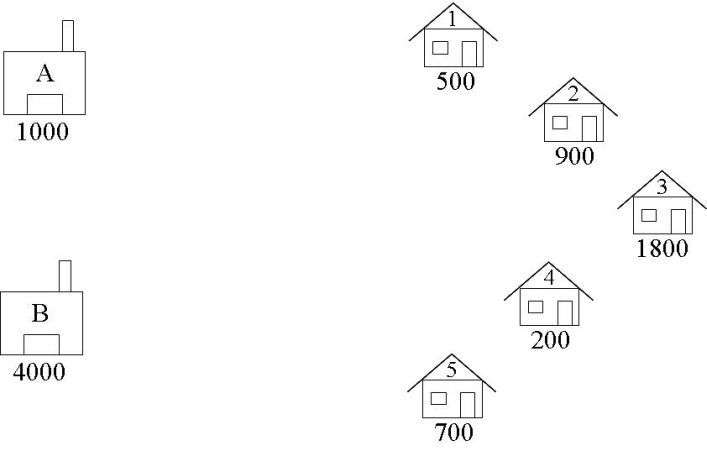
A boutique brewery has two warehouses from which it distributes beer to five carefully chosen bars. At the start of every week, each bar sends an order to the brewery’s head office for so many crates of beer, which is then dispatched from the appropriate warehouse to the bar. The brewery would like to have an interactive computer program which they can run week by week to tell them which warehouse should supply which bar so as to minimize the costs of the whole operation. For example, suppose that at the start of a given week the brewery has 1000 cases at warehouse A, and 4000 cases at warehouse B, and that the bars require 500, 900, 1800, 200, and 700 cases respectively. Which warehouse should supply which bar?

Formulation

For transportation problems, using a graphical representation of the problem is often helpful during formulation. Here is a graphical representation of The Beer Distribution Problem.

Identify the Decision Variables

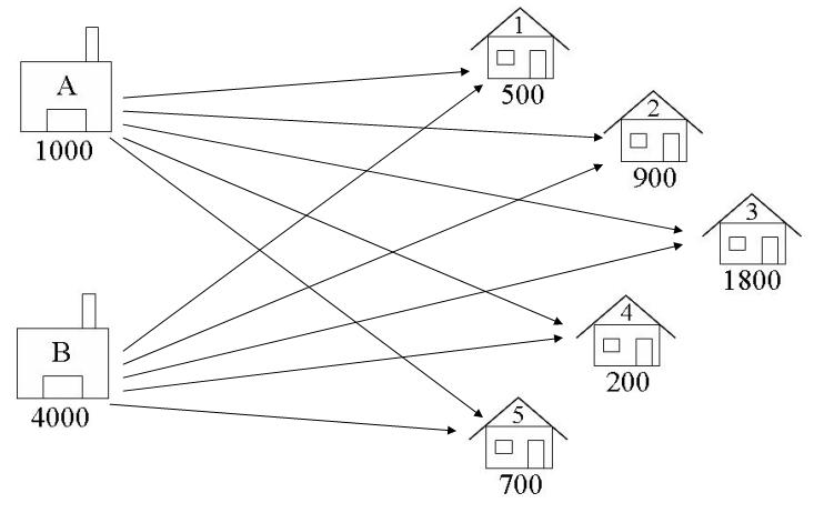
In transportation problems we are deciding how to transport goods from their supply nodes to their demand nodes. The decision variables are the Arcs connecting these nodes, as shown in the diagram below. We are deciding how many crates of beer to transport from each warehouse to each pub.

• A1 = number of crates of beer to ship from Warehouse A to Bar 1
• A5 = number of crates of beer to ship from Warehouse A to Bar 5
• B1 = number of crates of beer to ship from Warehouse B to Bar 1
• B5 = number of crates of beer to ship from Warehouse B to Bar 5

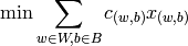
Let:

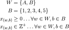
The lower bound on the variables is Zero, and the values must all be Integers (since the number of crates cannot be negative or fractional). There is no upper bound.

Formulate the Objective Function

The objective function has been loosely defined as cost. The problem can only be formulated as a linear program if the cost of transportation from warehouse to pub is a linear function of the amounts of crates transported. Note that this is sometimes not the case. This may be due to factors such as economies of scale or fixed costs. For example, transporting 10 crates may not cost 10 times as much as transporting one crate, since it may be the case that one truck can accommodate 10 crates as easily as one. Usually in this situation there are fixed costs in operating a truck which implies that the costs go up in jumps (when an extra truck is required). In these situations, it is possible to model such a cost by using zero-one integer variables: we will look at this later in the course.

We shall assume then that there is a fixed transportation cost per crate. (If the capacity of a truck is small compared with the number of crates that must be delivered then this is a valid assumption). Lets assume we talk with the financial manager, and she gives us the following transportation costs (dollars per crate):

From Warehouse to Bar	A	B
1	2	3
2	4	1
3	5	3
4	2	2
5	1	3

Minimise the Transporting Costs = Cost per crate for RouteA1 * A1 (number of crates on RouteA1)

+ ... + Cost per crate for RouteB5 * B5 (number of crates on RouteB5)

Formulate the Constraints

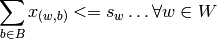
The constraints come from considerations of supply and demand. The supply of beer at warehouse A is 1000 cases. The total amount of beer shipped from warehouse A cannot exceed this amount. Similarly, the amount of beer shipped from warehouse B cannot exceed the supply of beer at warehouse B. The sum of the values on all the arcs leading out of a warehouse, must be less than or equal to the supply value at that warehouse:

Such that:

• A1 + A2 + A3 + A4 + A5 <= 1000
• B1 + B2 + B3 + B4 + B5 <= 4000

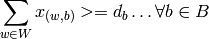
The demand for beer at bar 1 is 500 cases, so the amount of beer delivered there must be at least 500 to avoid lost sales. Similarly, considering the amounts delivered to the other bars must be at least equal to the demand at those bars. Note, we are assuming there are no penalties for oversupplying bars (other than the extra transportation cost we incur). We can _balance_ the transportation problem to make sure that demand is met exactly - there will be more on this later. For now, the sum of the values on all the arcs leading into a bar, must be greater than or equal to the demand value at that bar:

• A1 + B1 >= 500
• A2 + B2 >= 900
• A3 + B3 >= 1800
• A4 + B4 >= 200
• A5 + B5 >= 700

Finally, we have already specified the amount of beer shipped must be non-negative.

PuLP Model

Whilst the LP as defined above could be formulated into Python code in the same way as the A Blending Problem (Whiskas), for Transportation Problems, there is a more efficient way which we will use in this course. The example file for this problem is found in the examples directory BeerDistributionProblem.py

First, start your Python file with a heading and the import PuLP statement:

"""
The Beer Distribution Problem for the PuLP Modeller

Authors: Antony Phillips, Dr Stuart Mitchell    2007
"""

# Import PuLP modeller functions
from pulp import *

The start of the formulation is a simple definition of the nodes and their limits/capacities. The node names are put into lists, and their associated capacities are put into dictionaries with the node names as the reference keys:

# Creates a list of all the supply nodes
Warehouses = ["A","B"]

# Creates a dictionary for the number of units of supply for each supply node
supply = {"A": 1000,
        "B": 4000}

# Creates a list of all demand nodes
Bars = ["1", "2", "3", "4", "5"]

# Creates a dictionary for the number of units of demand for each demand node
demand = {"1": 500,
        "2": 900,
        "3": 1800,
        "4": 200,
        "5": 700}

The cost data is then inputted into a list, with two sub lists: the first containing the costs of shipping from Warehouse A, and the second containing the costs of shipping from Warehouse B. Note here that the commenting and structure of the code makes the data appear as a table for easy editing. The Warehouses and Bars lists (Supply and Demand nodes) are added to make a large list (of all nodes) and inputted into PuLPs makeDict function. The second parameter is the costs list as was previously created, and the last parameter sets the default value for an arc cost. Once the cost dictionary is created, if costs[“A”][“1”] is called, it will return the cost of transporting from warehouse A to bar 1, 2. If costs[“C”][“2”] is called, it will return 0, since this is the defined default.

# Creates a list of costs of each transportation path
costs = [   #Bars
        #1 2 3 4 5
         [2,4,5,2,1],#A  Warehouses
        [3,1,3,2,3] #B
         ]
}}}

The prob variable is created using the LpProblem function, with the usual input parameters.

# Creates the prob variable to contain the problem data
prob = LpProblem("Beer Distribution Problem",LpMinimize)

A list of tuples is created containing all the arcs.

# Creates a list of tuples containing all the possible routes for transport
Routes = [(w,b) for w in Warehouses for b in Bars]

A dictionary called route_var is created which contains the LP variables. The reference keys to the dictionary are the warehouse name, then the bar name([“A”][“2”]) , and the data is Route_Tuple. (e.g. [“A”][“2”]: Route_A_2). The lower limit of zero is set, the upper limit of None is set, and the variables are defined to be Integers.

# A dictionary called route_vars is created to contain the referenced variables (the routes)
route_vars = LpVariable.dicts("Route",(Warehouses,Bars),0,None,LpInteger)

The objective function is added to the variable prob using a list comprehension. Since route_vars and costs are now dictionaries (with further internal dictionaries), they can be used as if they were tables, as for (w,b) in Routes will cycle through all the combinations/arcs. Note that i and j could have been used, but w and b are more meaningful.

# The objective function is added to prob first
prob += lpSum([route_vars[w][b]*costs[w][b] for (w,b) in Routes]), "Sum of Transporting Costs"

The supply and demand constraints are added using a normal for loop and a list comprehension. Supply Constraints: For each warehouse in turn, the values of the decision variables (number of beer cases on arc) to each of the bars is summed, and then constrained to being less than or equal to the supply max for that warehouse. Demand Constraints: For each bar in turn, the values of the decision variables (number on arc) from each of the warehouses is summed, and then constrained to being greater than or equal to the demand minimum.

# The supply maximum constraints are added to prob for each supply node (warehouse)
for w in Warehouses:
    prob += lpSum([route_vars[w][b] for b in Bars]) <= supply[w], "Sum of Products out of Warehouse %s"%w

# The demand minimum constraints are added to prob for each demand node (bar)
for b in Bars:
    prob += lpSum([route_vars[w][b] for w in Warehouses]) >= demand[b], "Sum of Products into Bars %s"%b

Following this is the prob.writeLP line, and the rest as explained in previous examples.

You will notice that the linear programme solution was also an integer solution. As long as Supply and Demand are integers, the linear programming solution will always be an integer. Read about naturally integer solutions for more details.

Extensions

Validation

Since we have guaranteed the Supply and Demand are integer, we know that the solution to the linear programme will be integer, so we don’t need to check the integrality of the solution.

Storage and “Buying In”

Transportation models are usually _balanced_, i.e., the total supply = the total demand. This is because extra supply usually must be stored somewhere (with an associated storage cost) and extra demand is usually satisfied by purchasing extra goods from alternative sources (this is know as “buying in” extra goods) or by substituting another product (incurring a penalty cost).

In The Beer Distribution Problem, the total supply is 5000 cases of beer, but the total demand is only for 4100 cases. The extra supply can be sent to an _dummy_ demand node. The cost of flow going to the dummy demand node is then the storage cost at each of the supply nodes.

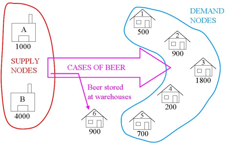
This is added into the above model very simply. Since the objective function and constraints all operated on the original supply, demand and cost lists/dictionaries, the only changes that must be made to include another demand node are:

# Creates a list of all demand nodes
Bars = ["1","2","3","4","5","D"]

# Creates a dictionary for the number of units of demand for each demand node
demand = {"1": 500,
            "2": 900,
            "3": 1800,
            "4": 200,
            "5": 700,
            "D": 900}

# Creates a list of costs of each transportation path
costs = [   #Bars
     #1 2 3 4 5 D
     [2,4,5,2,1,0],#A  Warehouses
     [3,1,3,2,3,0] #B
     ]

The Bars list is expanded and the Demand dictionary is expanded to make the Dummy Demand require 900 crates, to balance the problem. The cost list is also expanded, to show the cost of “sending to the Dummy Node” which is realistically just leaving the stock at the warehouses. This may have an associated cost which could be entered here instead of the zeros. Note that the solution could still be solved when there was an unbalanced excess supply.

If a transportation problem has more demand than supply, we can balance the problem using a dummy supply node. Note that with excess demand, the problem is “Infeasible” when unbalanced.

Assume there has been a production problem and only 4000 cases of beer could be produced. Since the total demand is 4100, we need to get extra cases of beer from the dummy supply node.

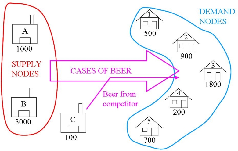
This dummy supply node is added in simply and logically into the Warehouse list, Supply dictionary, and costs list. The Supply value is chosen to balance the problem, and cost of transport is zero to all demand nodes.

# Creates a list of all the supply nodes
Warehouses = ["A","B","D"]

# Creates a dictionary for the number of units of supply for each supply node
supply = {"A": 1000,
      "B": 3000,
      "D": 100}

# Creates a list of all demand nodes
Bars = ["1","2","3","4","5"]

# Creates a dictionary for the number of units of demand for each demand node
demand = {"1": 500,
      "2": 900,
      "3": 1800,
      "4": 200,
      "5": 700}

# Creates a list of costs of each transportation path
costs = [   #Bars
     #1 2 3 4 5 D
     [2,4,5,2,1], #A
     [3,1,3,2,3], #B  Warehouses
     [0,0,0,0,0]  #D
     ]

Presentation of Solution and Analysis

There are many ways to present the solution to The Beer Distribution Problem: as a list of shipments, in a table, etc.

TRANSPORTATION SOLUTION -- Non-zero shipments
TotalCost = ____

Ship ___ crates of beer from warehouse A to pub 1
Ship ___ crates of beer from warehouse A to pub 5
Ship ___ crates of beer from warehouse B to pub 1
Ship ___ crates of beer from warehouse B to pub 2
Ship ___ crates of beer from warehouse B to pub 3
Ship ___ crates of beer from warehouse B to pub 4

This information gives rise to the following management summary:

The Beer Distribution Problem
Mike O'Sullivan, 1234567
We are minimising the transportation cost for a brewery operation. The brewery
transports cases of beer from its warehouses to several bars.

The brewery has two warehouses (A and B respectively) and 5 bars (1, 2, 3, 4 and
5).

The supply of crates of beer at the warehouses is:

__________

The forecasted demand (in crates of beer) at the bars is:

__________

The cost of transporting 1 crate of beer from a warehouse to a bar is given in
the following table:

__________

To minimise the transportation cost the brewery should make the following
shipments:

Ship ___ crates of beer from warehouse A to pub 1
Ship ___ crates of beer from warehouse A to pub 5
Ship ___ crates of beer from warehouse B to pub 1
Ship ___ crates of beer from warehouse B to pub 2
Ship ___ crates of beer from warehouse B to pub 3
Ship ___ crates of beer from warehouse B to pub 4

The total transportation cost of this shipping schedule is $_____.

Ongoing Monitoring

Ongoing Monitoring may take the form of:

• Updating your data files and resolving as the data changes (changing costs, supplies, demands);
• Resolving our model for new nodes (e.g., new warehouses or bars);
• Looking to see if cheaper transportation options are available along routes where the transportation cost affects the optimal solution (e.g., how much total savings can we get by reducing the transportation cost from Warehouse B to Bar 1).