Using OSInstance Methods: Low Level Calls

The code snippets used in this section are from the example code algorithmicDiffTest.cpp in the algorithmicDiffTest folder in the examples folder. The code is based on the following example.

$$\quad x_{0}^{2} + 9x_{1}$$ Minimize (20)

$$33 - 105 + 1.37 x_{1} + 2x_{3} + 5 x_{1} \le 10$$ s.t. (21)

$$\ln(x_{0} x_{3}) + 7x_{2} \ge 10$$ (22)

$$x_{0}, x_{1}, x_{2}, x_{3} \ge 0$$ (23)

The OSiL representation of the instance (20)-(23) is given in Appendix 14.3. This example is designed to illustrate several features of OSiL. Note that in constraint (21) the constant 33 appears in the <con> element corresponding to this constraint and the constant 105 appears as a <number> OSnL node in the <nonlinearExpressions> section. This distinction is important, as it will lead to different treatment by the code as documented below. There are no nonlinear terms in the instance that involve variable $x_{1}.$ The terms $5x_{1}$ in (21) and $7 x_{2}$ in (22) are expressed in the objectives and <linearConstraintCoefficients> sections, respectively, and will again receive special treatment by the code. However, the term $1.37x_1$ in (21), along with the term $2x_3$, is expressed in the <nonlinearExpressions> section. Variables $x_{1}$ and $x_{2}$ do not appear in any nonlinear terms. However, in the OSInstance API, variable $x_{1}$ appears in the <nonlinearExpressions> section; hence it is treated as a nonlinear variable for purposes of algorithmic differentiation. Variable $x_{2}$ never appears in the <nonlinearExpressions> section and is therefore treated as a linear variable and not used in any algorithmic differentiation calculations. Variables that do not appear in the <nonlinearExpressions> are never part of the algorithmic differentiation calculations.

Ignoring the nonnegativity constraints, instance (20)-(23) defines a mapping from $\mathbb{R}^{4}$ to $\mathbb{R}^{3}.$

$$\left[ \begin{array}{r} x_0^2+9x_1 \\ 33 - 105 + 1.37x_1 + 2x_3 + 5x_1 \\ \ln (x_0x_3) + 7x_2 \end{array}\right] = \left[ \begin{array}{r} 9x_1 \\ 33 + 5x_1 \\ 7x_2 \end{arra... ... \\ - 105 + 1.37x_1 + 2x_3 \\ \ln (x_0x_3) \end{array}\right]$$

$$= \left[ \begin{array}{r} 9x_1 \\ 33 + 5x_1 \\ 7x_2 \end{arra... ...begin{array}{r} f_1(x) \\ f_2(x) \\ f_3(x) \end{array}\right]$$

$$\hbox{\rm where}\ f(x) := \left[ \begin{array}{r} f_1(x) \\ f_2(x) \\ f_3(x) \end{array} \right]$$ (24)

The OSiL representation for the instance in (20)-(23) is read into an in-memory OSInstance object as follows (we assume that osil is a string with the OSiL instance)

osilreader = new OSiLReader();
osinstance = osilreader->readOSiL( &osil);

There is a method in the OSInstance class, initForAlgDiff() that is used to initialize the nonlinear data structures. A call to this method

osinstance->initForAlgDiff( );

will generate a map of the indices of the nonlinear variables. This is critical because the algorithmic differentiation only operates on variables that appear in the <nonlinearExpressions> section. An example of this map follows.

std::map<int, int> varIndexMap;
std::map<int, int>::iterator posVarIndexMap;
varIndexMap = osinstance->getAllNonlinearVariablesIndexMap( );
for(posVarIndexMap = varIndexMap.begin(); posVarIndexMap
	!= varIndexMap.end(); ++posVarIndexMap){
	std::cout <<  "Variable Index = "   << posVarIndexMap->first  << std::endl ;
}

The variable indices listed are 0, 1, and 3. Variable 2 does not appear in the <nonlinearExpressions> section and is not included in varIndexMap. That is, $f$ will be considered as a map from $\mathbb{R}^{3}$ to $\mathbb{R}^{3}.$

Once the nonlinear structures are initialized it is possible to take derivatives using algorithmic differentiation. Algorithmic differentiation is done using either a forward or reverse sweep through an expression tree (or operation sequence) representation of $f$. The two key public algorithmic differentiation methods in the OSInstance class are forwardAD and reverseAD. These are actually generic ``wrappers'' around the corresponding CppAD methods with the same signature. This keeps the OS API public methods independent of any underlying algorithmic differentiation package.

The forwardAD signature is

std::vector<double> forwardAD(int k, std::vector<double> vdX);

where $k$ is the highest order Taylor coefficient of $f$ to be returned, $\tt vdX$ is a vector of doubles in $\mathbb{R}^{n},$ and the function return is a vector of doubles in $\mathbb{R}^{m}.$ Thus, $k$ corresponds to the $k$ in Equations (12) and (14), where vdX corresponds to the $x^{(k)}$ in Equation (12), and the $y^{(k)}$ in Equation (14) is the vector in range space returned by the call to forwardAD. For example, by Equation (15) the following call will evaluate each component function defined in (24) corresponding only to the nonlinear part of (24) - the part denoted by $f(x)$.

funVals = osinstance->forwardAD(0, x0);

Since there are three components in the vector defined by (24), the return value funVals will have three components. For an input vector,

x0[0] = 1; // the value for variable x0 in function f
x0[1] = 5; // the value for variable x1 in function f
x0[2] = 5; // the value for variable x3 in function f

the values returned by osinstance->forwardAD(0, x0) are 1, -63.15, and 1.6094, respectively. The Jacobian of the example in (24) is

$$J = \left[ \begin{array}{rrrr} 2x_{0} &9.00&0.00&0.00 \\ 0.00&6.37&0.00&2.00 \\ 1/x_{0}&0.00&7.00&1/x_{3} \end{array}\right]$$ (25)

and the Jacobian $J_f$ of the nonlinear part is

$$J_f = \left[ \begin{array}{ccc} 2x_0 & 0.00 & 0.00 \\ 0.00 & 1.37 & 2.00 \\ 1/x_0 & 0.00 & 1/x_3 \end{array} \right]$$ (26)

When $x_{0} = 1,$ $x_{1} = 5,$ $x_{2} = 10,$ and $x_{3} = 5$ the Jacobian $J_f$

$$J_f = \left[ \begin{array}{ccc} 2.00 & 0.00 & 0.00 \\ 0.00 & 1.37 & 2.00 \\ 1.00 & 0.00 & 0.20 \end{array}\right]$$ (27)

A forward sweep with $k = 1$ will calculate the Jacobian column-wise. See (16). The following code will return column 3 of the Jacobian (27) which corresponds to nonlinear variable $x_{3}.$

x1[0] = 0;
x1[1] = 0;
x1[2] = 1;
osinstance->forwardAD(1, x1);

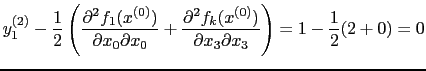
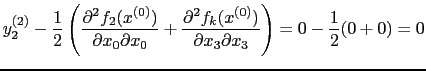
Now calculate second derivatives. To illustrate we use the results in (17)-(19) and calculate

$$\frac{\partial^2 f_{k}(x^{(0)})}{\partial x_{0} \partial x_{3}} \quad k = 1, 2, 3.$$

Variables $x_{0}$ and $x_{3}$ are the first and third nonlinear variables so by (18) the $x^{(1)}$ should be the sum of the $e^{(1)}$ and $e^{(3)}$ unit vectors and used in the first-order forward sweep calculation.

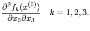x1[0] = 1;
x1[1] = 0;
x1[2] = 1;
osinstance->forwardAD(1, x1);

Next set $x^{(2)} = 0$ and do a second-order forward sweep.

std::vector<double> x2( n);
x2[0] = 0;
x2[1] = 0;
x2[2] = 0;
osinstance->forwardAD(2, x2);

This call returns the vector of values

$$y_{1}^{(2)} = 1, \quad y_{2}^{(2)} = 0, \quad y_{3}^{(2)} = -.52$$

By inspection of (26),

$$\frac{\partial^2 f_{1}(x^{(0)})}{\partial x_{0} \partial x_{0}} = 2$$

$$\frac{\partial^2 f_{2}(x^{(0)})}{\partial x_{0} \partial x_{0}} =$$ 0

$$\frac{\partial^2 f_{3}(x^{(0)})}{\partial x_{0} \partial x_{0}} = -1$$

$$\frac{\partial^2 f_{1}(x^{(0)})}{\partial x_{3} \partial x_{3}} =$$ 0

$$\frac{\partial^2 f_{2}(x^{(0)})}{\partial x_{3} \partial x_{3}} =$$ 0

$$\frac{\partial^2 f_{3}(x^{(0)})}{\partial x_{3} \partial x_{3}} = -.04$$

Then by (19),

$$\frac{\partial^2 f_{1}(x^{(0)})}{\partial x_{0} \partial x_{3}} = y_{1}^{(2)} - \frac{1}{2} \left( \frac{\partial^2 f_{1}(x^{(0)})}... ...}(x^{(0)})}{\partial x_{3} \partial x_{3}} \right) = 1 - \frac{1}{2}(2 + 0) = 0$$

$$\frac{\partial^2 f_{2}(x^{(0)})}{\partial x_{0} \partial x_{3}} = y_{2}^{(2)} - \frac{1}{2} \left( \frac{\partial^2 f_{2}(x^{(0)})}... ...}(x^{(0)})}{\partial x_{3} \partial x_{3}} \right) = 0 - \frac{1}{2}(0 + 0) = 0$$

$$\frac{\partial^2 f_{3}(x^{(0)})}{\partial x_{0} \partial x_{3}} = y_{3}^{(2)} - \frac{1}{2} \left( \frac{\partial^2 f_{3}(x^{(0)})}... ...0)})}{\partial x_{3} \partial x_{3}} \right) = -.52 - \frac{1}{2}(-1 - .04) = 0$$

Making all of the first and second derivative calculations using forward sweeps is most effective when the number of rows exceeds the number of variables.

The reverseAD signature is

std::vector<double> reverseAD(int k, std::vector<double> vdlambda);

where vdlambda is a vector of Lagrange multipliers. This method returns a vector in the range space. If a reverse sweep of order $k$ is called, a forward sweep of all orders through $k -1$ must have been made prior to the call.